Database page layouts

Just about every major database deals with memory in terms of pages. “Page” here refers to a continuous block of memory of fixed size that is typically a multiple of Linux kernel page size (historically, 4096B). Rows can be arranged within a page in various ways.

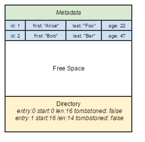
The granddaddy of all database page layouts is the NSM format, which most traditional RDBMSes use. Rows are appended sequentially to a page. Updates to a row are usually done by marking a tombstoned bit (or setting some snapshot identifier), following by appending the updated row.

NSM page format.

NSM page format.

  • Pros: Fastest write performance of all page layouts — simple sequential append to a logical file. Easy to access the whole row and return it. Lots of techniques to index the row itself exist.
  • Cons: Not easy to project on variable-length rows. SIMD performance not accessible on columns.

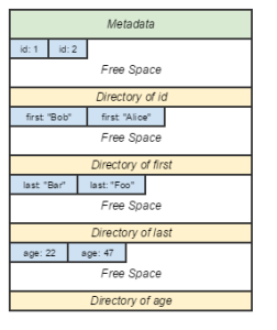
The traditional alternative to NSM is the DSM layout, which is the classical “column-oriented” database page layout. Individual elements within a row are teased out, and are grouped by their own columns.

Column-oriented DSM page layout.

Column-oriented DSM page layout.

It’s my belief that column-oriented databases sound amazing when one first hears of them, but think through them critically, and they’re not as amazing. Their classical advantage is in query performance — just slurp up a bunch of fixed-length elements while reading, maybe even load them to a SIMD register and perform calculations in parallel.

Except that… the overhead in splitting them up, storing them separately, and stitching columns back together is significant, especially when taking consistency in consideration. Whereas a row is the atomic block of consistency in NSM databases, the individual element is the atomic block in column-oriented stores.

The query performance advantage only applies to a narrow set of queries. It is non-trivial to do projections on columns that involve filtering on a separate column. It’s not surprising that HBase, probably the most widely used column-oriented database, advises against creating more than 2-4 “column families” (their terminology for separate groupings of elements). In short, the advantage of DSM is limited to a narrow set of queries that arguably do not see a lot of real world value.

  • Pros: Fast theoretical query & calculation performance. Possible improved update I/O performance due to not having to write the whole row on update.
  • Cons: Significant overhead in writes and reads of whole rows; consistency will add more overhead to queries due to a lower granularity to track. Best-case query & project scenarios are not necessarily common-case scenarios.

The PAX page layout groups rows by their constituent elements, on the same page.

PAX page layout.

  • Pros: Eliminates most of the major disadvantages of the DSM model.
  • Cons: Challenging implementation. Some disadvantages persist, they just don’t require hopping pages. Real-world performance data lacking.

In addition to the above three formats, an endless variety exist. Fractured mirrors take advantage of replication to combine multiple page layouts and to try and have the best of all worlds. NoSQL databases typically implement some variety of the above, or use their own format. HBase, for instance, records its updates to a WAL and otherwise keeps its rows in a memory cache, and flushes batches to an “immutable” logical file sorted by row identifier.
Posted in Databases | Tagged | Leave a comment

Simplified database consistency, Part 1: Obligatory CAP Theorem musings

Brewer’s Conjecture was formalized as the CAP theorem when this paper was published. It’s a good read. In this blog entry, I will talk about my philosophical take on the CAP theorem.

Let’s break down the three letters of the CAP Theorem.

  • Consistency – This represents the “correctness” of a database.
  • Availability – This represents the ability of a database to serve requests in a performant manner.
  • Partition Tolerance – This represents the ability of a database to operate with node or net failure.

The CAP theorem is commonly stated as “pick any two, you can’t have the third one.” In reality, there’s a tension between all points of the CAP triangle, and each edge in the triangle is a nebulous continuum. First, let’s break down what “consistency” really means.

The defining standard of a consistent database is ACID. I will restate it slightly differently for programmers who may not be database architects:

A database which follows ACID constructs will have the same state as a database that has a global read-write lock on the entire system, with the property that any unexpected write failure results in rollback of all changes before the write lock is released.

(This isn’t quite accurate, but is good enough for this blog.)

Obviously, we can’t have a global read-write lock in most scenarios: we’d be sacrificing too much availability. So, how do we achieve the appearance of a single global read-write lock while serving all requests fast enough? My contention is: you can’t. If it walks like a duck, if it quacks like a duck — then it’s a duck. The only way to achieve highest consistency levels is to have a global read-write lock or something just as inefficient. Therein lies the most obvious A-C tradeoff.

From there, the tension between A-C is a continuum which I would state as: “the more the system has to synchronize on, the more availability that is traded off.” NoSQL databases often describe themselves as fully “AP” or fully “CP”; in practice, “CP” and “AP” are meaningless descriptions, and it is intractable for a database to achieve either full availability or full consistency.

To simplistically demonstrate this continuum, consider these following assertions:

  • If a transaction relies on record-level consistency, then record locks are needed.
  • If a transaction relies on a range of rows being consistent, then multiple record locks are needed.
  • If a transaction relies on a table being consistent, then table locks are needed.
  • If a transaction relies on multiple tables being consistent, then multi-table locks are needed.

In addition to the above, if any of these applies over a distributed system, then there has to be some sort of global lock/synchronization/consensus dance which is hard to execute efficiently. Even the Paxos algorithm relies on the existence of some global monotonically increasing sequence to be perfect, which brings its own set of tradeoffs.

There are ways to push back on having actual write locks, usually at the expense of space: for instance, it’s possible to avoid non-repeatable reads without acquiring a table lock in a NSM format database (that is, append-only records; every update is a tombstone followed by an append of a new record) simply by tagging records with a timestamp, then note the current timestamp at the start of a read, and not reading any records with a timestamp above the current timestamp. But these pushbacks are effective only to a point; we don’t want to be creating a copy of a table to achieve table-level consistency, for instance.

What about the “P” component, partition tolerance? If one thinks of “P” as not just network partitions, but as network latency, out of order messages, and so on, then it becomes apparent that P cannot be code-sacrificed in a distributed system, simply because partitions are always ongoing to some degree or another in a distributed system. The only databases which can be honestly described as anywhere near “AC” are traditional RDBMSes.

One might be tempted to think of NoSQL databases such as Cassandra as pushing the end of the AP triangle. But there’s more to the rabbit hole. Column-oriented stores are the true extreme end of the AP triangle, breaking down record-level consistency to element-level consistency. More on this in Part II.

Posted in Databases | Tagged , | Leave a comment

Simplified database consistency, Part 0: Not-so-simplified reference tables

A proper Database Theory 101 class would begin with the CAP Theorem – that it is impossible to have consistency, availability, and partition tolerance in the same database. This is a first in a blog series explaining the CAP theorem and all its nuances, and how it applies to distributed databases.

Part 0 starts out with reference material with minimal explanation, because I spent a lot of time putting together definitions from various sources to one place, and I’d like it in the cloud instead of my aging stack of filled notebooks.

The real Part I will go back to the basics: the CAP theorem and how it has been proven.

Database anomalies (sometimes called “phenomena”), which I sourced from various points:

Anomaly Name Description
Dirty Read Transaction T1 can read uncommitted data from a different transaction T2.
Non-Repeatable Read / Fuzzy Read Two reads within the same transaction T1 are not guaranteed to contain the same data within rows due to transaction T2 having been executed a write to these rows in between.
Phantom Read Two queries within the same transaction T1 return different rows due to transaction T2 having inserted or deleted rows in between.
Read Skew T1 reads a row x. T2 then modifies rows x and y, and commits. T1 then reads modified y, which may have been dependent on a row x that had not been committed at a time. (Classic example: calculating bank balances)
Dirty Write Two transactions change the same record at the same time.
Lost Updates Two transactions update the same row. The transaction that did the update first is now lost and was never seen by the other transaction.
Write Skew Two transactions concurrently read an overlapping data set, make disjoint updates, and then commit without seeing updates. For example: A bank has a rule that the combined balance of an user’s accounts must be 0 or greater. An user with 2 accounts has a balance of $100 each for a total of $200. With write skew, the user can initiate simultaneous withdrawals of $200 from each account, withdrawing $400 total, which is not detected because each individual transaction thinks the net balance is $200.
Real-Time Violation Transaction T1 sees transaction t2, but not necessarily all of the transactions that have occurred before t2. Applicable to a replicated distributed database.
Forward Freshness Applicable to replicated distributed databases, T1 is started before T2. T2 is considered committed by the database, and T1 is allowed to read data from T2, meaning that T1 does not actually read off a “snapshot” at the time it started. Opacity is lost.

Table of isolation levels defined by ANSI/ISO SQL:

Isolation Level Locks Acquired Disallowed Phenomenons
READ UNCOMMITTED Write lock on record only for duration of operation N/A
READ COMMITTED Write lock on record for duration of transaction Dirty reads
REPEATABLE READ Both read and write locks acquired on affected rows for duration of transaction Non-repeatable reads
SERIALIZABLE Range locks for duration of transaction Phantom reads


The next two tables are mostly from this paper which was quite influential in my old company. Extended consistency levels in distributed databases:

Continue reading »

Posted in Databases | Tagged , | Leave a comment

Using tf-idf to measure emoji sentiment

My data scientist friend suggested two changes to the emoji/emoticon script I wrote: sort the list by score, and use tf-idf to calculate the significance of a detected emoticon and emoji and filter on that.

tf-idf stands for “term frequency, inverse document frequency.” The idea is that if a term appears a lot in a document (tweet), then that term must be important. But if the term also appears in a lot of documents, then it must be not-so-important. Here’s the pseudocode to calculate a tf-idf score for each given word in a document:

let tf = number of times the word appears in the document / number of words in a document
let n_containing = the number of documents where the word appears
let idf = math.log(number of documents) / (1 + n_containing)
let tf-idf = tf * idf

To calculate the average tf-idf of a word for all tweets, I took the median of the tf-idf score for tweets that did contain that particular term.

To adopt the definition of a word for purposes of counting emojis as words in a tweet, I used the following regular expression and counted the occurrence of each within the tweet:

\S+

I expanded the tweet list to 16K, and then filtered for terms that appeared more than 20 times and had an average tf-idf of 0.01. The only pre-processing I did within the tweet was to substitute any whitespace, including newlines, for a single space.

Here’s the new list — much nicer! Thanks for the suggestions, Michael!

Term Sentiment Score TD-IDF Occurrences Positive Score Negative Score
5.32 0.040 28 151 -2
5.09 0.023 22 114 -2
? 4.58 0.059 26 119 -0
4.52 0.099 21 99 -4
? 3.73 0.032 37 138 -0
? 3.50 0.026 42 173 -26
? 3.39 0.012 101 358 -16
? 3.07 0.027 30 112 -20
‘. 2.56 0.016 32 90 -8
? 2.44 0.022 50 145 -23
😉 2.36 0.035 22 52 -0
?? 2.23 0.044 22 63 -14
£ 2.18 0.026 28 67 -6
?. 2.00 0.020 29 58 -0
? 2.00 0.020 29 58 -0
? 2.00 0.040 58 116 -0
? 2.00 0.020 29 58 -0
? 2.00 0.020 29 58 -0
? 2.00 0.020 29 58 -0
? 2.00 0.040 58 116 -0
= 1.72 0.031 29 89 -39
? -1.58 0.023 31 47 -96
| 1.56 0.012 79 175 -52
.@ 1.52 0.017 40 96 -35
@__ 1.46 0.033 28 79 -38
“@ 1.41 0.023 27 65 -27
?! 1.39 0.026 28 67 -28
? -1.37 0.035 30 22 -63
~ 1.36 0.024 39 84 -31
1.21 0.017 38 77 -31
? -1.18 0.042 22 26 -52
!!!! 1.08 0.036 36 75 -36
?? 1.06 0.020 51 120 -66
? 1.05 0.049 20 33 -12
?? -0.99 0.014 70 97 -166
__: -0.98 0.023 41 47 -87
] 0.94 0.013 67 114 -51
? -0.87 0.037 23 26 -46
[ 0.79 0.014 61 96 -48
__ 0.70 0.016 60 129 -87
??? -0.66 0.013 85 101 -157
🙁 0.61 0.026 31 64 -45
??? 0.55 0.051 20 44 -33
.” 0.51 0.018 37 53 -34
* 0.51 0.013 184 295 -202
? -0.42 0.023 52 77 -99
….. 0.41 0.020 37 68 -53
? -0.39 0.043 23 46 -55
???? 0.33 0.041 21 40 -33
? 0.29 0.017 51 84 -69
? -0.29 0.039 31 52 -61
;& -0.25 0.016 116 126 -155
0.25 0.033 36 57 -48
-0.22 0.021 27 44 -50
?” 0.03 0.018 30 48 -47
Posted in Programming | Tagged | Leave a comment

Getting Twitter sentiment of emoticons and emoji

A data scientist friend and I talked briefly about how hard it is to parse text into words. He mentioned that he felt that not enough attention were paid to emoticons or emoji in the Twitter sentiment analysis papers he reads.

In this context, a sentiment score is a measure of emotion associated with a word or phrase. Negative scores mean the word is associated with negative emotions, and positive scores mean the word is associated with positive emotions.

Coincidentally, I’d been taking a data science course, and the assignment I was working on concerned Twitter sentiment analysis. It wasn’t too hard to adopt the homework to estimate sentiment for non-alphanumeric characters. The regular expression I used to grab emoticons and emoji was:

[^A-Za-z0-9\s]+

Clearly, the above regex captures more than emoticons and emoji — it captures valid words in non-ASCII languages and punctuation. Nonetheless, I thought it’d be an interesting start.

For calculating the score of nonalphanumeric sentiments, the formula I used was:

let pos = [cumulative score of positive sentiment words of the tweet which the term appeared in]
let neg = [cumulative score of negative sentiment words of the tweet which the term appeared in]
let count = [number of times that terms appeared in the document]
let sentiment = pos / count - neg / count

Where the sentiment words and scores are taken from the AFINN list.

I did a quick and dirty run through about 6K English tweets collected from the Twitter sprinkler API. Not a representative sample by any means, but again, my aim was to get a quick estimate, not a scientific paper. The results are below — terms which appeared fewer than 10 times are not published here.

Term Sentiment Score Occurrences Positive Score Negative Score
@ 1.41 2629 6337 -2630
. 1.19 2585 5816 -2733
: 0.99 1746 3770 -2033
/ 1.14 1470 3014 -1341
:// 1.07 1421 2871 -1349
0.61 1119 2503 -1816
# 1.74 753 1795 -483
, 1.22 692 1723 -877
_ 1.56 421 1013 -355
! 2.59 356 1111 -190
1.67 315 835 -310
1.27 265 538 -201
0.57 255 498 -353
? 1.55 197 482 -177
; 0.97 188 447 -265
& 1.13 151 400 -230
0.60 122 234 -161
!! 2.17 114 352 -105
( 1.09 76 133 -50
) 1.01 68 112 -43
_: -0.28 58 95 -111
@_ 0.19 57 117 -106
.. 0.75 52 115 -76
2.11 46 131 -34
? 0.33 43 84 -70
;& 0.66 38 53 -28
❤️ 3.24 37 129 -9
* 0.79 34 65 -38
!!! 2.73 30 100 -18
🙂 2.93 27 98 -19
? 4.04 25 106 -5
?? 1.58 24 64 -26
[ 0.95 22 40 -19
] 0.64 22 36 -22
$ 1.95 22 62 -19
??? 0.05 21 22 -21
…. -0.05 21 30 -31
.” 0.05 19 23 -22
? 4.78 18 86 0
5.00 18 90 0
| 2.41 17 44 -3
?? -1.12 16 25 -43
0.27 15 33 -29
__ 1.29 14 34 -16
% 1.43 14 26 -6
? 2.54 13 42 -9
0.69 13 24 -15
+ 2.25 12 33 -6
? 4.33 12 54 -2
:… 2.45 11 32 -5
? 0.18 11 20 -18
??? 4.00 11 44 0
0.36 11 20 -16
? -0.40 10 11 -15
__: 0.90 10 23 -14
? 2.80 10 32 -4
Posted in Programming | Tagged | Leave a comment

On Java threads and Linux

Yesterday, I asked a seemingly simple question: What is a Java thread?

In Linux, the concept of a thread is ambiguous. Schedulable units are created through clone, which defines familiar options such as sharing the same thread group (CLONE_THREAD) or sharing the same address spaces (CLONE_VM). The options span about a dozen items, defining I/O context sharing, file descriptors, signal handlers, and so on. The fork call defines few shared options, while pthread_create uses more shared context.

Does Java use pthread_create, fork, or its own variant of clone, or even its own userspace implementation? Java VMs obviously are free to differ in their implementations, but I had to sate my own curiosity regardless.

Continue reading »

Posted in Linux | Tagged , , | Leave a comment

Tax Liens Part IV: What happened

The lien auction was online, and register bidders could compete with each other, just like eBay.  Being a seasoned eBay veteran and former consigner’s assistant, I knew to wait until the last day of the auction to start sniping.

Continue reading »

Posted in Investing | Tagged , | Leave a comment

Intermission: What are tax liens?

The feedback I’ve gotten so far has been: “uh, what are tax liens?”  Here, I backtrack to explain what tax liens are.

Continue reading »

Posted in Investing | Tagged | Leave a comment

Tax Liens Part III: Deciding how much to bid

In Part II, I narrowed down a list of thousands of liens to roughly 30 I wanted to bid on.  Now came the hard part: how much should I bid for these liens?

I built a Monte Carlo simulator that took in several parameters:

  • Number of liens
  • Average lien price
  • Average premium percentage
  • Number of iterations to simulate

Looking at the chart from Part I, there is a roughly 15% percent chance that the lien is never redeemed by the property owner.  Yet, Colorado claims transfer of deed happens in less than one percent of all purchases.  How can that be?  I believe this is because most elect to not to go through the transfer of deed, because the lien they end up with is a dead end property as described in Part II.  Since I narrowly targeted properties, this was not a concern for me.  I thus marked liens that went past 40+ months as a “transfer of deed” with a conservative $15,000 return.

Still, this didn’t sit well with me even though El Paso’s statistics clearly indicated a nontrivial number of liens remained unredeemed past 40+ months.  So, in the simulator, I separated the “non-house” iterations from those that “won” a house to give me a better view of what would happen if all of my liens would be redeemed.

So my output looked like this for 7 liens, $1200 each, 8% premium, 10000 iterations:

Over 10000 iterations:
Average outlay: $18693.12
Subtaxed the next year: 3.96 Pct: 0.57%
Average profit: $17459.30; 93.40%
Number of losing iterations: 36; 0.36%
Number of iterations without houses: 3822; 38.22%
Average outlay (no house only): $17640.92
Average profit (no house only): $1331.01; 7.55%
Number of losing iterations (no house only): 36; 0.94%

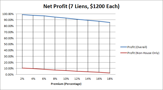
Here’s an Excel graph of estimated profits over increasing premiums using the same inputs, divided between house and non-house:

Net profit on tax liens

The net profit I would make on tax liens, with and without the assumption I’d get a transfer of deed.

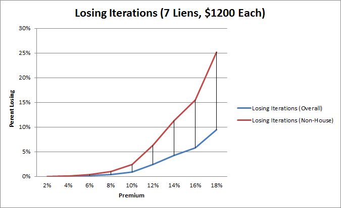
Another view, the percentage of time I would lose out:


Losing iterations

Percentage of the time I would lose money on a tax lien.

Obviously, the premium played a big factor into the “riskiness” of the tax liens and the net profit I’d make on them.  We agreed to bid up to 10% on them, as that still had a low chance that we’d lose out plus they would yield a generous 6.57% on average even if we wound up with no transfer of deed.

Now it was time to bid!  Part IV covers what happened at the auction and thereafter.  You may download my crappy Perl code if you wish, here: tax_lien_monte_cristo

Posted in Investing | Tagged , | Leave a comment

Tax Liens Part II: Picking out the targets

Part I describes how I derived an estimated rate of redemption from my liens. Next came determining which liens to buy; there were thousands to choose from.  Time to start building a script.

The goal, obviously, is to maximize returns on liens.  There are two ways to lose out on liens:

  1. Property owner redeems the lien too early.  This scenario was covered in Part I — the interest rate accrues at 0.83% monthly, and so in order to make a profit, the lien must be held for as many months as it takes to overtake the premium.
  2. Property owner never redeems the lien on an unprofitable property.  In Colorado, when a property is passed to a lienholder, it comes free of most debts including mortgage debts, so responsibility for old debts is usually not a worry.  Rather, the worry is that the lienholder could end up with a property that is unable to be turned over for a profit — for instance, a house that is actually a hollowed-out meth factory or more commonly, a parcel of desert land no one would ever buy.

Looking through the list of available properties showed a surprise: many property owners were corporations, businessmen, or real estate speculators.

Continue reading »

Posted in Investing | Tagged , | Leave a comment
« Older